


Next: 4.6 Supercell calculations
Up: 4. Implementation
Previous: 4.4 Algorithms and practicalities
Contents
Subsections
4.5 Pseudopotentials
The inclusion of core
electrons poses special problems in QMC calculations distinct from
those encountered in other electronic structure methods. The differing
timescale (or equivalently distance scale) on which the electrons move
compared with valence electrons requires the use of special
modified sampling schemes or the use of very small timesteps which reduce
the efficiency of the simulation. Large ionic and kinetic
energies in the core regions are a further problem. Although
accurate wavefunctions may be constructed for low  atoms,4.7 for high atoms accurate
wavefunctions have yet to be designed and obtained.
atoms,4.7 for high atoms accurate
wavefunctions have yet to be designed and obtained.
These two difficulties conspire to focus computational effort on the
core electrons, forcing attention away from the chemically interacting
and physically interesting valence and bonding regions. Fortunately
for many properties of interest, and for many materials, the core
remains almost independent of its environment and may be substituted
by a pseudopotential with negligible loss of accuracy.4.8 This
replacement serves to reduce the effective of the atoms that must
be dealt with. The -dependence in the scaling of QMC calculations
is then determined by the number of valence electrons that must be
included in order to obtain satisfactory results.
Pseudopotentials are used routinely in DFT and quantum chemical
applications and consequently there exists a large literature and
continued research effort on the
subject. [54,55,56,57,58,59,60,61]
Improvements to the pseudopotential approximation are not an aim of
this work: accurate potentials exist for carbon and silicon, the main
atomic species used. The pseudopotentials user were generated within
LDA-DFT. Evaluation of the pseudopotentials requires techniques
particular to QMC, and these are described in the remainder of the
section.
The pseudopotentials modify the many-body Hamiltonian, replacing the
electron-ion coulomb terms with
 |
(4.34) |
where  signifies the electron-ion dependent terms of ion
 , and
, and
 and
and
 are respectively a
long-ranged local potential and a short-ranged non-local
potential. The two potentials are chosen within a pseudopotential
construction scheme to accurately model the valence electrons. At
long-range, typically of order 2-3 a.u., the local potential returns
to the Coulomb tail.
are respectively a
long-ranged local potential and a short-ranged non-local
potential. The two potentials are chosen within a pseudopotential
construction scheme to accurately model the valence electrons. At
long-range, typically of order 2-3 a.u., the local potential returns
to the Coulomb tail.
The non-local potentials are written in terms of several short-ranged
angular momentum dependent potentials. The operator
is
given by these potentials multiplied by the appropriate projection
operators, written as integrals over the angular interval  :
:
 |
(4.35) |
The local component of the pseudopotential may be directly evaluated
during a Monte Carlo simulation. In supercell simulations, Ewald's
method (see section 4.6.1) is required to deal with the
long-range of the potential, but this this not a significant
complication. In VMC, the non-local potentials must be projected onto
the trial function which requires statistical evaluation of the
projection operators.
4.5.1.1 Evaluation of the non-local energy
Evaluation of the non-local projection operators, and hence
the non-local energy cannot be performed analytically. For general
correlated wavefunctions, the projection operators depend on all
inter-particle distances and are therefore not amenable to analytic or
numerical integration. Fahy [38,26]
developed an exact scheme for evaluating the non-local energy in VMC and
first applied the technique in simulations of bulk carbon and
silicon in the diamond structure. This scheme is now used almost
exclusively, approximate evaluation methods having been discarded due
to insufficient accuracy.
In the Fahy scheme, evaluation of
 is
performed stochastically during a VMC simulation. The projection is
written in terms of ratios of the trial function,
is
performed stochastically during a VMC simulation. The projection is
written in terms of ratios of the trial function,
 |
(4.36) |
where the sum  runs over all
  electrons at distances
  from the ion. The orientation of the coordinate system (which is
arbitrary) is chosen for each electron so that the vector
from the ion. The orientation of the coordinate system (which is
arbitrary) is chosen for each electron so that the vector  lies along the
  -direction, thus eliminating the
 -dependence of the integrals. [26]
The angular integral over
 is performed
stochastically during the simulation. Optimised integration grids have
been developed to exactly integrate functions of up to a certain
angular momentum. [62] The variance of the
estimator for the non-local energy is chosen to optimise the balance of
work spent evaluating the non-local pseudopotential with the work
performing other parts of the simulation. The grids are very
efficient, and in calculations on bulk silicon and carbon, taking
multiple samples of a grid was always found to be less efficient than
using a single larger grid. This result is expected to be general; the
integrals are effectively of low dimensionality and grid-based
integration methods should converge more rapidly than Monte Carlo
methods. In practice, 6-12 points give sufficient accuracy for first
and second row elements, [26,63] where the
character of the wavefunctions is dominated by
is performed
stochastically during the simulation. Optimised integration grids have
been developed to exactly integrate functions of up to a certain
angular momentum. [62] The variance of the
estimator for the non-local energy is chosen to optimise the balance of
work spent evaluating the non-local pseudopotential with the work
performing other parts of the simulation. The grids are very
efficient, and in calculations on bulk silicon and carbon, taking
multiple samples of a grid was always found to be less efficient than
using a single larger grid. This result is expected to be general; the
integrals are effectively of low dimensionality and grid-based
integration methods should converge more rapidly than Monte Carlo
methods. In practice, 6-12 points give sufficient accuracy for first
and second row elements, [26,63] where the
character of the wavefunctions is dominated by  and
and  angular-momenta. 6 point grids are sufficient to exactly integrate
 momenta, and 12 points grids,
  momenta.
The non-locality of accurate pseudopotentials is a significant problem
in DMC calculations. An explicit form for the many-body wavefunction
is not available in DMC and it has been shown
(e.g. Ref. [64]) that the matrix elements of the
non-local operator for imaginary time diffusion are negative. This
creates a sign problem similar to the sign problem of fermion
DMC. This problem has been avoided by replacing the non-local
potential operator by an approximate local potential determined
by evaluating the full non-local operator on the trial wavefunction,
as in VMC. [65,66] This approximation
has been shown to converge quadratically to the exact energy as the
trial wavefunction improves. [63] In practice this
approximation is very good and is not overly sensitive to details of
the trial function. The ``locality approximation'' results in a
non-variational DMC energy.
Core polarisation potentials (CPPs) are a refinement of
pseudopotential theory particularly designed for use in many-body
calculations. The pseudopotentials most commonly used in many-body
calculations are derived from mean field calculations. This represents
an approximation at some level, and to consistently achieve an
accuracy better than  eV on atomic energy levels, some
many-body effects must be incorporated into the pseudopotential.
eV on atomic energy levels, some
many-body effects must be incorporated into the pseudopotential.
Direct methods of generating pseudopotentials within QMC have met with
little success due to the difficulties in performing accurate
all-electron calculations of sufficient statistical
accuracy. [67]. Methods based on configuration
interaction calculations and quasiparticle calculations have met with
most
success. [60,68,69,70]
The accuracy of pseudopotentials may be increased by taking into
account the polarisability of the core, which is one of the most
important effects excluded by a conventional rigid core approach. It
is has been shown that this incorporates the leading terms of ``core
relaxation'', the change that a core undergoes in different chemical
environments (Ref. [71] and references within). The
formulation of CPPs considers the polarisation of the atomic core by
the valence electrons, within a point-dipole picture. To avoid
divergences in the potential, the effect fields experienced by valence
electrons are truncated close to the core. By parameterising the
truncation, the correct binding energies of valence electrons is
ensured. The scheme includes some of the core-core, core-valence and
valence-valence correlation effects of an all-electron, many-body
calculation. [71,68]
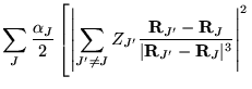
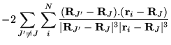
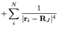
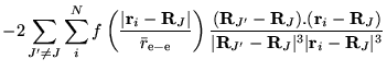
The many-body Hamiltonian is initially modified to include additional
CPP terms resulting from the polarisation induced electric
fields[68]
where  is the core polarisability, and the sums run over
all ions,
is the core polarisability, and the sums run over
all ions,  , and electrons. The terms are due to ion-ion,
ion-ion-electron, electron-ion and electron-electron-ion interactions
respectively. The electron dependent terms are further parameterised,
by means of a cutoff function, removing the
, and electrons. The terms are due to ion-ion,
ion-ion-electron, electron-ion and electron-electron-ion interactions
respectively. The electron dependent terms are further parameterised,
by means of a cutoff function, removing the  divergences:
 |
(4.38) |
where  is a rescaled coordinate. The Hamiltonian terms become
where  is the projection operator for angular momentum
 , and the
  and
and
 are parameters obtained
during construction of the CPP.[68]
are parameters obtained
during construction of the CPP.[68]
These terms may be directly evaluated within VMC and DMC. The
non-local projection operator, , is evaluated at the same
time as non-local component of the full pseudopotential, avoiding
costly evaluations of the many-body wavefunction.
Sample data
comparing DMC results for the ionisation potentials of a Ti atom for
different pseudopotentials [61] is given in Table
4.1.
Table 4.1:
Ionisation potentials of Ti
for several pseudopotentials computed using DMC. Energies are in eV
and statistical error bars are given in brackets. Experimental data
from [72]. Rel-TM denotes a relativistic
pseudopotential constructed in the Troullier-Martins
scheme, [58] HF and HF+CPP denote a bare HF
pseudopotential and an HF pseudopotential with core-polarisation
potential terms respectively. [68] The
pseudopotentials were generated in the configuration suggested by
G. B. Bachelet et al.[56] Data courtesy
Y. Lee [61]
| IP |
Expt |
Rel-TM |
HF |
HF+CPP |
|
|
|
| 1st |
6.82 |
6.862(15) |
6.693(13) |
6.767(16) |
|
|
|
| 2nd |
13.58 |
12.347(8) |
12.218(8) |
13.639(9) |
|
|
|
| 3rd |
27.48 |
27.666(4) |
28.288(4) |
28.413(5) |
|
|
|
| 4th |
43.24 |
44.336(0) |
44.774(0) |
46.228(0) |
|
|
|
|
Next: 4.6 Supercell calculations
Up: 4. Implementation
Previous: 4.4 Algorithms and practicalities
Contents
© Paul Kent
![$\displaystyle +\left.\sum_{i}^{N}\sum_{i^{\prime}\neq i}^{N}
\frac{({\bf r}_{i^...
...ime}-{\bf R}_{J}\vert^{3}\vert{\bf r}_{i}-{\bf R}_{J}\vert^{3}} \right] \;\;\;,$](pkthimg412.gif)
![$\displaystyle +\left.\sum_{i}^{N}\sum_{i^{\prime}\neq i}^{N}
f\left(\frac{\vert...
...ime}-{\bf R}_{J}\vert^{3}\vert{\bf r}_{i}-{\bf R}_{J}\vert^{3}} \right] \;\;\;,$](pkthimg419.gif)